Gausian Process Regression with Covariance Product and Sum

The atmospheric CO2 concentration readings in parts per million (ppm) by volume from air samples are collected continuously by the Mauno Loa observatory in Hawaii. The data are freely available at ftp: // ftp.cmdl.noaa.gov/ccg/co2/trends/. http://scrippsco2.ucsd.edu/data/atmospheric_co2/mlo

This example was first presented in the book of Rasmussen & Williams [1] and serves as a tutorial for kernel composition, see for instance - https://docs.pymc.io/notebooks/GP-MaunaLoa.html - https://scikit-learn.org/stable/auto_examples/gaussian_process/plot_gpr_co2.html - http://dfm.io/george/current/user/hyper/

The modelling and the SDE representation of Arno Solin and Simo Särkkä [2], which differs from the book of Rasmussen & Williams [3], is used here.

[1]

Rasmussen, C. E. & Williams, C. K. I. (2006), Gaussian Processes for Machine Learning , MIT Press

[2]

Arno Solin and Simo Särkkä (2014). Explicit link between periodic covariance functions and state space models. In Proceedings of the Seventeenth International Conference on Artifcial Intelligence and Statistics (AISTATS 2014). JMLR: W&CP, volume 33.

[3]

Rasmussen, C. E. & Williams, C. K. I. (2006), Gaussian Processes for Machine Learning , MIT Press

import matplotlib.pyplot as plt
import numpy as np
import pandas as pd

from pysip.regressors import Regressor
from pysip.statespace import Matern32, Matern52, Periodic

Load and prepare the Mauna Loa CO2 data set

df = pd.read_csv(
    "../../../data/mauna_loa/monthly_in_situ_co2_mlo.csv",
    comment='"',
    header=0,
    skipinitialspace=True,
)

df = df[["Date.1", "CO2"]].set_index("Date.1")
df.index.name = "Date"
df = df[df.CO2 != -99.99]

# Use data until 2010 for the fit and the rest for the prediction
C02_mean = df["CO2"].mean()
df["CO2_fit"] = df["CO2"] - C02_mean
df["CO2_pred"] = df["CO2_fit"]
df["CO2_pred"][df.index >= 2010] = np.nan

Initialize parameters and models

# Matérn 5/2 for slow rising trend (long-term effects)
p1 = [
    dict(name="mscale", value=2.295e03, transform="log"),
    dict(name="lscale", value=4.864e02, transform="log"),
    dict(name="sigv", value=2.210e-01, transform="log"),
]

# Periodic * Matérn 3/2 for quasi-periodic variations
p2 = [
    dict(name="period", value=1.0, transform="fixed"),
    dict(name="mscale", value=2.833e00, transform="log"),
    dict(name="lscale", value=1.341e00, transform="log"),
    dict(name="sigv", value=0.0, transform="fixed"),
]

p3 = [
    dict(name="mscale", value=1.0, transform="fixed"),
    dict(name="lscale", value=2.607e02, transform="log"),
    dict(name="sigv", value=0.0, transform="fixed"),
]

# Matérn 3/2 for short-term effects
p4 = [
    dict(name="mscale", value=4.595e-01, transform="log"),
    dict(name="lscale", value=6.359e-01, transform="log"),
    dict(name="sigv", value=0.0, transform="fixed"),
]

k1 = Matern52(p1, name="k1")
k2 = Periodic(p2, name="k2")
k3 = Matern32(p3, name="k3")
k4 = Matern32(p4, name="k4")

# Compose covariance function
K = k1 + k2 * k3 + k4
K

GPSum(hold_order=0, method='mfd', name='k1__+__k2__x__k3__+__k4')

Initialize the regressor

reg = Regressor(K, outputs="CO2_fit")

Do the frequentist fit

fit_summary, corr_matrix, opt_summary = reg.fit(df=df)
fit_summary

tnew = np.arange(1958, 2030, 0.01)
ds = reg.predict(df=df, smooth=True, tnew=tnew)

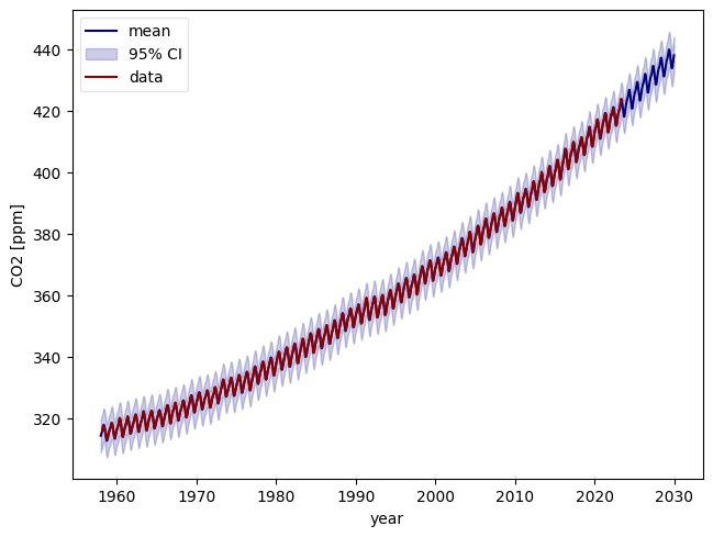
# Plot output mean and 95% credible intervals
ym = ds["y_mean"].sel(outputs="CO2_fit")
ysd = ds["y_std"].sel(outputs="CO2_fit")


plt.plot(tnew, C02_mean + ym, color="navy", label="mean")
plt.fill_between(
    tnew,
    C02_mean + ym - 2 * ysd,
    C02_mean + ym + 2 * ysd,
    color="darkblue",
    alpha=0.2,
    label=r"95% CI",
)
plt.plot(df.index, df["CO2"], color="darkred", label="data")
plt.tight_layout()
plt.legend(loc="best", fancybox=True, framealpha=0.5)
ax = plt.gca()
ax.set_xlabel("year")
ax.set_ylabel("CO2 [ppm]")

Text(38.347222222222214, 0.5, 'CO2 [ppm]')